A Pragmatic Introduction to Neural Networks for Software Engineers

TL;DR

Neural networks are systems of interconnected nodes (neurons) organized in layers, learning by adjusting connection weights via backpropagation. They excel at pattern recognition in complex data. This guide covers core concepts, implementation patterns in PyTorch, training strategies, and practical considerations for developers.

1. Core Concepts: The Building Blocks

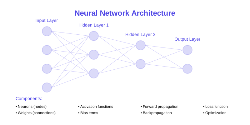
Neural networks are computational models inspired by biological nervous systems. They process information through layers of interconnected "neurons."

1.1. Neurons and Layers

• Neuron (Node): The fundamental processing unit. It receives inputs, applies a transformation (weighted sum + bias), and passes the result through an activation function.
• Layers: Neurons are organized into layers.
  • Input Layer: Receives raw data features. The number of neurons equals the number of input features.
  • Hidden Layers: Intermediate layers that perform feature extraction and transformation. The number of hidden layers and neurons per layer are hyperparameter choices.
  • Output Layer: Produces the network's prediction. The number of neurons and activation function depend on the task (e.g., one neuron with sigmoid for binary classification,
    N
    neurons with softmax for
    N
    -class classification).

1.2. Connections and Weights

• Connections: Links between neurons in adjacent layers.
• Weights: Parameters associated with each connection. They represent the strength and direction of the signal from one neuron to another. Learning in a neural network is primarily the process of adjusting these weights.
• Bias: An additional learnable parameter for each neuron (except input layer). It shifts the activation function's output, allowing for more flexible modeling.

1.3. Activation Functions

Non-linear functions applied to the output of each neuron (after the weighted sum and bias). They introduce non-linearity, enabling networks to learn complex patterns beyond linear relationships.

• Rectified Linear Unit (ReLU):
  • Formula:
    f(x) = max(0, x)
  • Pros: Computationally efficient, helps mitigate vanishing gradients.
  • Cons: "Dying ReLU" problem where neurons can become inactive.
• Sigmoid:
  • Formula:
    f(x) = 1 / (1 + exp(-x))
  • Pros: Smooth, output is in
    (0, 1)
    , useful for binary classification output.
  • Cons: Prone to vanishing gradients, not zero-centered.
• Hyperbolic Tangent (Tanh):
  • Formula:
    f(x) = tanh(x)
  • Pros: Smooth, output is in
    (-1, 1)
    , zero-centered.
  • Cons: Still prone to vanishing gradients.

1.4. Loss Functions

Quantify the difference between the network's predictions and the actual target values. The goal of training is to minimize this loss.

• Mean Squared Error (MSE):
  • Formula:
    L = 1/N * sum((y_true - y_pred)^2)
  • Use Case: Regression problems.
• Binary Cross-Entropy:
  • Formula:
    L = -1/N * sum(y_true * log(y_pred) + (1 - y_true) * log(1 - y_pred))
  • Use Case: Binary classification problems.
• Categorical Cross-Entropy:
  • Use Case: Multi-class classification problems (when targets are one-hot encoded).

2. Network Architecture and Implementation (PyTorch Example)

A typical feedforward neural network (Multilayer Perceptron - MLP) can be defined using PyTorch.

import torch
import torch.nn as nn
import torch.nn.functional as F

class FeedForwardNetwork(nn.Module):
    def __init__(self, input_dim, hidden_dims, output_dim, activation_fn=nn.ReLU()):
        """
        Initializes a feedforward neural network.

        Args:
            input_dim (int): The number of input features.
            hidden_dims (list of int): A list specifying the number of neurons in each hidden layer.
            output_dim (int): The number of output neurons.
            activation_fn (torch.nn.Module): The activation function to use between layers.
                                              Defaults to ReLU.
        """
        super(FeedForwardNetwork, self).__init__()
        
        layers = []
        current_dim = input_dim
        
        # Build hidden layers
        for h_dim in hidden_dims:
            layers.append(nn.Linear(current_dim, h_dim))
            layers.append(activation_fn)
            current_dim = h_dim
            
        # Output layer
        layers.append(nn.Linear(current_dim, output_dim))
        
        self.network = nn.Sequential(*layers)

    def forward(self, x):
        """
        Defines the forward pass of the network.

        Args:
            x (torch.Tensor): The input tensor.

        Returns:
            torch.Tensor: The output tensor.
        """
        return self.network(x)

# Example Usage:
input_features = 784  # e.g., flattened MNIST image
hidden_layer_sizes = [128, 64]
num_classes = 10

model = FeedForwardNetwork(input_features, hidden_layer_sizes, num_classes)
print(model)

# Example input
dummy_input = torch.randn(1, input_features) # Batch size of 1
output = model(dummy_input)
print(f"Output shape: {output.shape}")

3. Training: Learning from Data

Training involves iteratively adjusting network weights to minimize the loss function.

3.1. Forward and Backward Pass

1. Forward Pass: Input data flows through the network, layer by layer, producing an output prediction.
2. Loss Calculation: The loss function compares the prediction to the ground truth.
3. Backward Pass (Backpropagation): The error (loss) is propagated backward through the network. Gradients of the loss with respect to each weight and bias are computed using the chain rule of calculus.

3.2. Optimization

• Gradient Descent: An iterative optimization algorithm that moves in the direction of the steepest descent (negative gradient) of the loss function to find a minimum.
• Optimizers: Algorithms that implement gradient descent with various strategies to improve convergence speed and stability.

import torch.optim as optim

# Define model, loss function, and optimizer
model = FeedForwardNetwork(input_features, hidden_layer_sizes, num_classes)
criterion = nn.CrossEntropyLoss() # Suitable for multi-class classification
optimizer = optim.Adam(model.parameters(), lr=0.001, weight_decay=1e-5) # Adam optimizer with L2 regularization

# --- Training Loop Snippet ---
def train_epoch(model, data_loader, optimizer, criterion, device):
    model.train()  # Set model to training mode
    total_loss = 0
    for batch_x, batch_y in data_loader:
        batch_x, batch_y = batch_x.to(device), batch_y.to(device)

        optimizer.zero_grad() # Clear previous gradients

        outputs = model(batch_x)
        loss = criterion(outputs, batch_y)

        loss.backward()      # Backpropagation: compute gradients
        optimizer.step()     # Update weights

        total_loss += loss.item()
    return total_loss / len(data_loader)

def validate_epoch(model, data_loader, criterion, device):
    model.eval()  # Set model to evaluation mode
    total_loss = 0
    with torch.no_grad(): # Disable gradient calculation for validation
        for batch_x, batch_y in data_loader:
            batch_x, batch_y = batch_x.to(device), batch_y.to(device)
            outputs = model(batch_x)
            loss = criterion(outputs, batch_y)
            total_loss += loss.item()
    return total_loss / len(data_loader)

# Example training execution (requires DataLoaders 'train_loader', 'val_loader' and 'device')
# epochs = 10
# for epoch in range(epochs):
#     train_loss = train_epoch(model, train_loader, optimizer, criterion, device)
#     val_loss = validate_epoch(model, val_loader, criterion, device)
#     print(f"Epoch {epoch+1}/{epochs}, Train Loss: {train_loss:.4f}, Val Loss: {val_loss:.4f}")

4. Advanced Techniques & Architectures

4.1. Regularization

Techniques to prevent overfitting (when the model performs well on training data but poorly on unseen data).

• Dropout: During training, randomly sets a fraction of neuron outputs to zero for each forward pass. This forces the network to learn more robust features.

  class DropoutNetwork(nn.Module):
      def __init__(self, input_dim, hidden_dim, output_dim, dropout_prob=0.5):
          super(DropoutNetwork, self).__init__()
          self.fc1 = nn.Linear(input_dim, hidden_dim)
          self.dropout = nn.Dropout(dropout_prob)
          self.fc2 = nn.Linear(hidden_dim, output_dim)
  
      def forward(self, x):
          x = F.relu(self.fc1(x))
          x = self.dropout(x) # Apply dropout after activation
          x = self.fc2(x)
          return x
  

• Weight Decay (L2 Regularization): Adds a penalty term to the loss function proportional to the square of the weights. Encourages smaller weights, leading to a simpler model. Implemented directly in many optimizers (e.g.,
  weight_decay
  argument in
  optim.Adam
  ).
• Batch Normalization: Normalizes the inputs to a layer for each mini-batch. Stabilizes training, allows for higher learning rates, and can act as a regularizer.

4.2. Convolutional Neural Networks (CNNs)

Specialized for grid-like data, primarily images. They use convolutional layers to automatically learn spatial hierarchies of features.

• Convolutional Layer: Applies learnable filters to input data to detect local patterns (edges, textures).
• Pooling Layer: Downsamples feature maps, reducing spatial dimensions and computational complexity, while retaining important information. Max pooling is common.

class SimpleCNN(nn.Module):
    def __init__(self, num_classes=10):
        super(SimpleCNN, self).__init__()
        # Assuming input images are 1 channel (grayscale), 28x28 pixels (like MNIST)
        self.conv1 = nn.Conv2d(in_channels=1, out_channels=32, kernel_size=3, stride=1, padding=1)
        self.pool = nn.MaxPool2d(kernel_size=2, stride=2) # Reduces dimensions by half
        # After conv1 (28x28) and pool, output is 32 channels, 14x14
        self.fc1 = nn.Linear(32 * 14 * 14, 128)
        self.fc2 = nn.Linear(128, num_classes)

    def forward(self, x):
        x = self.pool(F.relu(self.conv1(x))) # Conv -> Activation -> Pool
        x = x.view(-1, 32 * 14 * 14)        # Flatten for fully connected layers
        x = F.relu(self.fc1(x))
        x = self.fc2(x)
        return x

# Example CNN usage:
cnn_model = SimpleCNN(num_classes=10)
print(cnn_model)

# Example input (Batch size 1, 1 channel, 28x28 image)
dummy_image_input = torch.randn(1, 1, 28, 28)
cnn_output = cnn_model(dummy_image_input)
print(f"CNN Output shape: {cnn_output.shape}")

5. Data Preparation and Preprocessing

Crucial for successful training.

• Normalization/Standardization: Scaling features to a similar range (e.g.,
  [0, 1]
  or zero mean, unit variance) is vital for stable gradient updates.

  def normalize_data(data):
      # Assuming data is a PyTorch tensor or NumPy array
      mean = data.mean(axis=0) # Calculate mean per feature
      std = data.std(axis=0)   # Calculate std per feature
      # Avoid division by zero for features with no variance
      std[std == 0] = 1e-8
      normalized_data = (data - mean) / std
      return normalized_data
  

• Splitting Data: Divide dataset into training, validation, and test sets.
  • Training Set: Used to train the model (adjust weights).
  • Validation Set: Used to tune hyperparameters and monitor for overfitting during training.
  • Test Set: Used for a final, unbiased evaluation of the trained model's performance.
• Data Loaders: PyTorch's
  DataLoader
  provides efficient batching, shuffling, and parallel data loading.

from torch.utils.data import DataLoader, TensorDataset

# Assuming you have your training features 'X_train' and labels 'y_train' as PyTorch tensors
# Convert to TensorDataset and then DataLoader
train_dataset = TensorDataset(X_train_tensor, y_train_tensor)
train_loader = DataLoader(train_dataset, batch_size=64, shuffle=True)

val_dataset = TensorDataset(X_val_tensor, y_val_tensor)
val_loader = DataLoader(val_dataset, batch_size=64, shuffle=False)

6. Practical Considerations and Best Practices

• Start Simple: Begin with a minimal architecture and gradually increase complexity if performance is insufficient.
• Hyperparameter Tuning: Learning rate, batch size, number of layers/neurons, activation functions, and regularization strengths significantly impact performance. Use the validation set for tuning.
• Monitor Training: Track training and validation loss/accuracy. Look for divergence or stagnation.
• Early Stopping: Halt training when validation performance stops improving (or starts degrading) to prevent overfitting.
• Debugging:
  • Gradient Checking: Ensure gradients are flowing correctly (not vanishing or exploding).
    None
    gradients often indicate issues.
  • Activation Visualization: Inspecting activation outputs can reveal if neurons are saturated or dead.
  • Sanity Checks: Train on a very small subset of data or with randomized labels to ensure the model can overfit this simpler case.

# Debugging Helper: Check for None gradients
def check_gradients_exist(model):
    for name, param in model.named_parameters():
        if param.requires_grad and param.grad is None:
            print(f"Warning: Gradient is None for parameter {name}")

7. Trade-offs

• Model Complexity vs. Data Size: More complex models require more data to train effectively without overfitting.
• Training Time vs. Model Performance: Deeper/wider networks and extensive hyperparameter search increase training time but can yield better results.
• Regularization Strength: Higher regularization reduces overfitting but can lead to underfitting if too aggressive.
• Choice of Activation Function: ReLU is fast but can suffer from dying neurons; others avoid this but are computationally more expensive or prone to vanishing gradients.
• Optimizer Choice: Adam often converges faster than SGD but can sometimes generalize slightly worse. SGD with momentum can be very effective with careful tuning.

8. When Not to Use Neural Networks

• Small Datasets: For very small datasets, simpler models like linear regression, logistic regression, or decision trees often perform better and are less prone to overfitting.
• Tabular Data with Clear Relationships: If relationships between features are well-understood and can be modeled with traditional statistical methods or rule-based systems, NNs might be overkill.
• Interpretability is Paramount: Standard neural networks are often "black boxes." If a highly interpretable model is required (e.g., for regulatory compliance), consider linear models, decision trees, or rule-based systems.
• Limited Computational Resources for Inference: Very deep or wide networks can be computationally expensive for real-time or embedded applications.
• Need for Guarantees: NNs provide empirical performance; they don't offer formal guarantees like some classical algorithms in specific domains.

9. Decision Checklist

• Problem Type: Is it classification, regression, generation, or another task suited for NNs?
• Data Availability: Do you have sufficient labeled data? Is it representative?
• Data Complexity: Are the patterns in the data linear or highly non-linear?
• Computational Budget: Do you have the resources for training and inference?
• Interpretability Requirements: Is a "black box" model acceptable, or is explainability crucial?
• Alternative Models: Have simpler models been considered and found insufficient?
• Domain Knowledge: Can domain expertise guide feature engineering or model architecture choices?

---

Resources

• PyTorch Official Documentation
• TensorFlow Official Documentation
• Deep Learning by Ian Goodfellow, Yoshua Bengio, and Aaron Courville: www.deeplearningbook.org
• Michael Nielsen, Neural Networks and Deep Learning: neuralnetworksanddeeplearning.com
• fast.ai - Practical Deep Learning for Coders